Introduction:
In this assignment, you will use R to examine and build models and significance tests for the speech recognition error data discussed in the Goldwater et al. paper.
Getting the data
We provide in the data zip file, 3 data files and an R file for reading them in and normalizing things a bit. In terms of the paper, this will get you to the end of section 2. As usual, I seem to be the man of the big data sets. But this one isn't as bad as last time. There's only 42 MB of data....
If you're in the goldwater directory created when you unpack the data, you can load all the data by giving the command source("process_data.r"). Look at the bottom of that script to see what you get. There are multiple data frames, paired for each of the two systems sri and cam. The two most useful ones, in terms of the analyses done in the paper are sri_full and sri_rescaled (and the corresponding files for the Cambridge data).
If you've got a large, new data set, often a good place to start is the summary() command, which will tell you about the variables in the data frame, their types and range of values.
- The column
is_errsays whether any sort of recognition error is attributed to that particular word. This is true if it was deleted or substituted by the speech recognizer or there was an insertion by the speech recognizer adjacent to it. - The column
rergives the IWER discussed in section 2. It is usually 1 or 0, corresponding to a deletion or substitution, but may have real values less than or greater than 1 if there is a single or multiple insertion errors adjacent to it.
Q1
Do simple exploratory data analyses for two variables and how they affect word error rate. That'll usually mean producing some sort of plot. Choose one categorical and one numeric variable. We'll do one for gender (you should choose two others). The second page of the paper cited work showing a higher error rate for men in speech rec systems. I decided on a simple mosaic plot for this binary variable
attach(sri_full)
mosaicplot(is_err ~ sex, main="SRI error by gender")
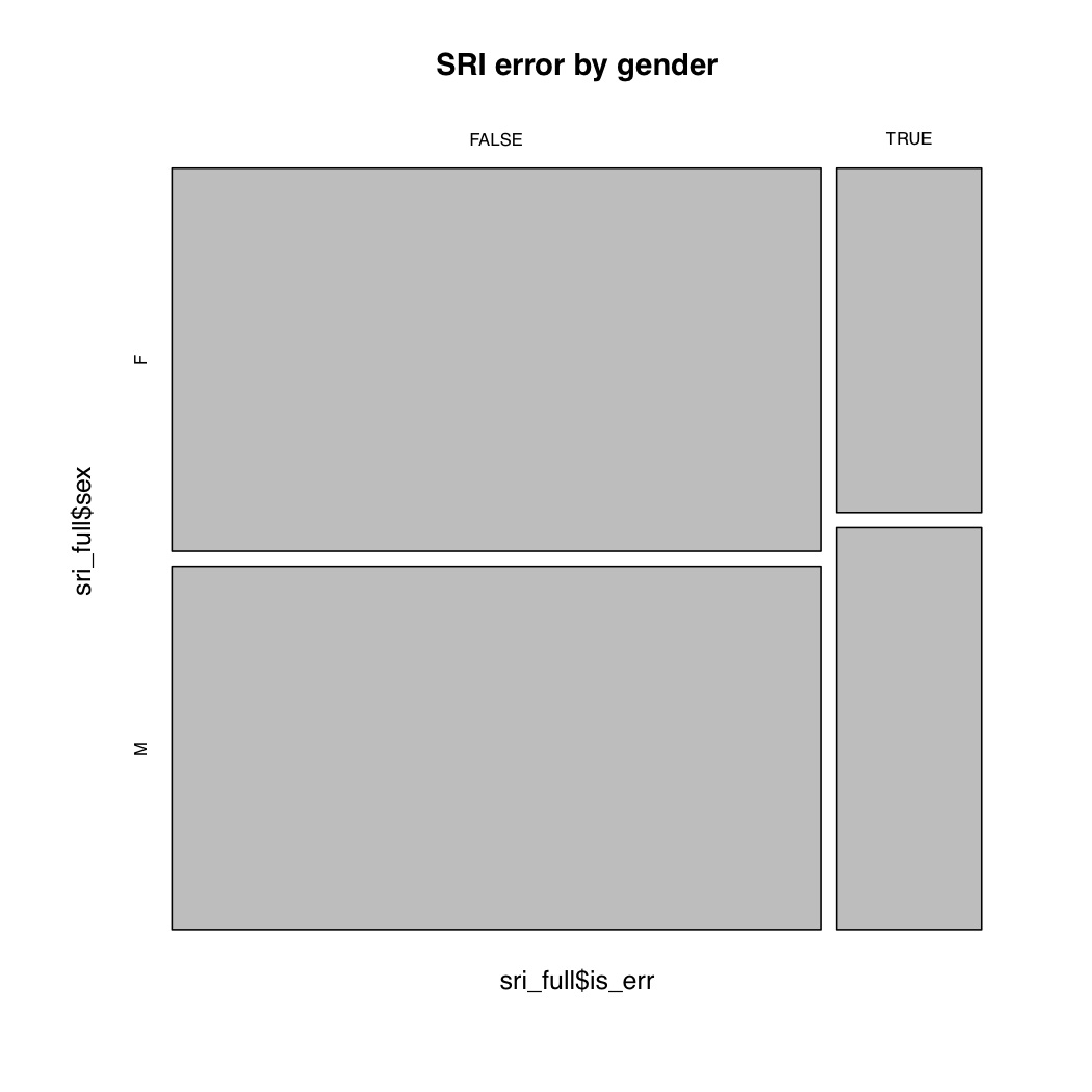
The SRI data indeed follows the pattern of more errors for male speakers. For getting statistics of something else by the levels of a factor, a good command to know is tapply(), which will make a table giving a function of one column by the levels of another. For example, for word length, look at the output of:
tapply(cam_full$is_err, cam_full$wlen_c, mean)
You should be able to plot that!
Q2
At various times when the other guys have let me, I've mentioned (approximate) permutation tests, and how I think they are conceptually simple, computer science friendly, and in principle usually better. If you don't like integrals, approximate permutation tests are for you! You can see the Wikipedia page. They were what was used to generate significance levels in table 4. There are R packages for such tests (not surprisingly!), such as MChtest, but they're easy enough to code up by hand, and it's probably a good way to really understand them. So let's do just that. Let's check the result that each speech recognizer is significantly less likely to make an error on the word after a repetition. Here's what we do:
- For the data set of n data items, there is some difference in the error rate (rer) between data items after a repetition and all other data items diff, and there is some number of data items after a repetition k.
- We'll have a for loop. The paper did it 10,000 times, though you could make it a bit smaller.
- We then want to work out the chance that if you randomly chose k samples from the n, what proportion of the time would the calculated difference in error rates for samples in and outside the k be greater than or equal to the observed diff. If this number is low, then the difference is significant
- To permute the data, you'll want to know about the sample() command. In it's simplest usage, it'll just permute your data for you!
- You then look at the error rate in the first k samples versus the rest and see how it compares to diff.
- Work out the proportion of the time the difference in IWER is as big or bigger in the samples, and that gives you a significance level!
Write code to do this and give the significance levels you calculate for both SRI and Cambridge. (They should be similar to the values in the paper, but not identical, of course. Though actually the values I'm getting for one system are a bit higher than those reported in the paper for reasons that I'm not quite sure of. Hmm....)
Q3
Build some logistic regression models for predicting speech recognition errors on words. As in the paper, the response variable will be is_err, and I suggest using the cam_rescaled and sri_rescaled, since as well as rescaling the data, there is some other clean up (filling in features, deleting outliers, ...) between cam_full and cam_rescaled.
Let's K.I.S.S. Rather than use either the Design package or lme4 for mixed effects models, as in the paper, let's build some simply logistic regression models, using R's standard built-in generalized linear models routine glm(). For this, the response variable will be is_err and the data frames will be the rescaled ones, and it's essential that you specify family="binomial" to get a logistic regression. If you're foggy on logistic regression in general or for R in particular, you might look at this handout, which I wrote for another course. (In terms of the discussion in that handout, we have "long format" data (one row per data item), but as noted towards the beginning of section 3, you can use that sort of data within glm().
- Pick a bunch of predictors (say, 10-20). Build a model for both SRI and Cam. Use the summary() function on it to see the details (perversely!). You might also use anova(), which, when applied to the output of a glm, gives you a G2 test of the change in deviance (-2 × LL) for adding each factor in turn.
- Drop the non-significant predictors from each model, and build a second model for each data set.
Q4
Reproduce the graph in figure 8. That tapply() command that I mentioned earlier can be usefully used here too! Who is that guy in the upper right corner? What value do you calculate for the r2 for this distribution? If this pattern is true in general, what does this say about speech recognition systems?
Collaboration policy: You may
collaborate providing you make sure you still learn something.
Submission guidelines:
Your submission should consist of an email to the
staff mailing list. Incude an attachment with the R code you used for each question, suid.r and a document with the plots and discussion answering the questions suid.pdf. Thanks!